Role of the P-Curve analysis in understanding publication bias
Publication bias is an effect of questionable research practices that have been corrupted the published record. One example of phenomena when scientists tend to publish studies supporting their hypothesis and putting aside those that do not are called the file-drawer problem (Rosenthal, 1979). The method to measure the extent of this corruption is to assess the meta-analytic collection of significant p-values, so-called p-curve analysis (Simonson et al., 2014).
In this post, we discuss how to draw a p-curve for the set of observed values to examine whether a given set of significant findings is merely the result of selective reporting.
First, we simulated the database (Wickham et al. 2019; Youngflesh 2018):
## load libraries
library(tidyverse)
## ── Attaching packages ─────────────────────────────────────── tidyverse 1.3.1 ──## ✓ ggplot2 3.3.3 ✓ purrr 0.3.4
## ✓ tibble 3.1.1 ✓ dplyr 1.0.5
## ✓ tidyr 1.1.3 ✓ stringr 1.4.0
## ✓ readr 1.4.0 ✓ forcats 0.5.1## ── Conflicts ────────────────────────────────────────── tidyverse_conflicts() ──
## x dplyr::filter() masks stats::filter()
## x dplyr::lag() masks stats::lag()library(MCMCvis)
library(ggridges) # https://cran.r-project.org/web/packages/ggridges/vignettes/introduction.html
library(ggpubr) # https://rpkgs.datanovia.com/ggpubr/
library(extraDistr) # https://github.com/twolodzko/extraDistr##
## Attaching package: 'extraDistr'## The following object is masked from 'package:purrr':
##
## rduniflibrary(pwr) # https://github.com/heliosdrm/pwr
set.seed(12)
N <- 100 # number of studies for PW
N_a <- 76 # number of articles
ef <- 0.3 # the true effect for PW (small effects)
tau_e <- 0.15 # the standard deviation of the true effects for studies
tau_a <- 0.1 # the standard deviation of the true effects for articles
SE <- 0.1 # the standard deviation of the sampling distribution
# the probability to publish the study based the p-value
w_publish <- c(0.2, 0.5, 1) # (0.10, 1] (0.05, 0.10] [0, 0.05]
sd_e <- rnorm(N, 0, tau_e) # studies
sd_a <- rnorm(N_a, 0, tau_a) # articles
df_simu <- tibble(
article = c(sample(1:N_a, N_a),
sample(1:N_a, N-N_a, replace = T)),
seTE = rtnorm(N, 0.25, SE, a = 0)) %>%
arrange(article) %>%
mutate(TE = rnorm(n(), ef+sd_e+sd_a[article], SE), #
studlab = paste0("E",1:n()),
article = paste0("A",article),
pvalue = round((1-pnorm(abs(TE), 0, SE))*2, 3))
df_simu## # A tibble: 100 x 5
## article seTE TE studlab pvalue
## <chr> <dbl> <dbl> <chr> <dbl>
## 1 A1 0.0217 0.287 E1 0.004
## 2 A1 0.302 0.757 E2 0
## 3 A2 0.338 0.286 E3 0.004
## 4 A3 0.345 0.322 E4 0.001
## 5 A4 0.262 -0.211 E5 0.035
## 6 A5 0.132 0.292 E6 0.003
## 7 A6 0.343 0.206 E7 0.04
## 8 A7 0.226 0.338 E8 0.001
## 9 A8 0.284 0.292 E9 0.004
## 10 A9 0.219 0.0982 E10 0.326
## # … with 90 more rowsP-curve analysis
To conduct a p-curve analysis, we can use the ‘pcurve’ function from the ‘dmetar’ package (Harrer et al. 2019).
## load package
library(dmetar)
## Registered S3 methods overwritten by 'lme4':
## method from
## cooks.distance.influence.merMod car
## influence.merMod car
## dfbeta.influence.merMod car
## dfbetas.influence.merMod car## Extensive documentation for the dmetar package can be found at:
## www.bookdown.org/MathiasHarrer/Doing_Meta_Analysis_in_R/## p-curve function
pcurve(df_simu)## Warning: Unknown or uninitialised column: `I2`.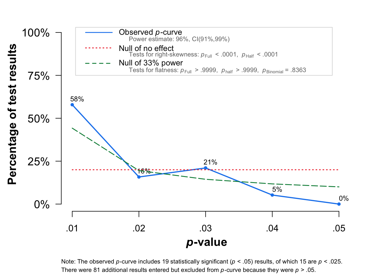
## P-curve analysis
##  -----------------------
## - Total number of provided studies: k = 100
## - Total number of p<0.05 studies included into the analysis: k = 19 (19%)
## - Total number of studies with p<0.025: k = 15 (15%)
##
## Results
##  -----------------------
##                     pBinomial  zFull pFull  zHalf pHalf
## Right-skewness test     0.010 -9.084     0 -8.778     0
## Flatness test           0.836  6.325     1  9.681     1
## Note: p-values of 0 or 1 correspond to p<0.001 and p>0.999, respectively.
## Power Estimate: 96% (90.5%-98.8%)
##
## Evidential value
##  -----------------------
## - Evidential value present: yes
## - Evidential value absent/inadequate: no
Output
The first output provides information about:
A. P-curve analysis
This section of the output shows general details about the studies used for the p-curve analysis.
B. Results
This section displays the results of the Right-Skewness test and the Flatness tests. The Right-Skewness test analyzes if the p-curve resulting from our data is significantly right-skewed, which should be expected if a “true” effect is behind our data. The flatness test analyzes if the p-curve is significantly flat, which indicates insufficient power or lack of “true” effect behind our data. For both tests, result are reported for the full p-curve (p < .05; zFull & pFull) and for the half-curve (p < .025; zHalf & pHalf).
C. Power Estimates
It tells us about the estimated power of the studies in our analysis.
D. Evidential value
It is the most important part of the output which provides an interpretation of the Results section. There are two types of information provided [1] if the evidential value is present (the desired answer for “true” effect is ‘yes’) and [2] if it is absent/inadequate (the desired answer for “true” effect is ‘no’).
P-Curve plot
The figure shows the p-curve for results when the p-values were between .01 and .05 (in blue).
The interpretation of the p-curve is very intuitive. If there is no effect, the distribution of the p-value should be uniform (red line). If there is a true effect, the distribution should be right-skewed, with more values close to the p = .01 and fewer values close to p = .05.
The p-curve distribution is also related to the power of studies included in the analysis. If we have enough power (the rule of thumb is 80% of power), we should expect a steeper slope of p-curve. In our case 74% of the time the significant effects are for p < .02.
If the effect reported in the literature is a subject of questionable research practice, we would observe left-skewed function with more significant effects closer to p = .05.
Limitations
The presented p-curve analyses method has some constraints. Specifically, p-curve estimates are not robust in the case of a small number of effect sizes and when the true effect sizes are heterogeneous. There are some promising developments, such as analyses of p-uniform to enable accurate effect size estimation in the presence of heterogeneity in true effect size (van Aert & van Assen, 2020).
Other promising developments are Bayesian methods to correct for publication bias (Du et al., 2017; Guan & Vandekerckhove, 2016) and the increased attention for the selection model approach (Citkowicz & Vevea, 2017; McShane et al., 2016). Here, we would like to explore in more detail the Robust Bayesian Meta-Analysis (RoBMA) proposed recently by Bartoš and Maier (2020).
Robust Bayesian Meta-Analysis (RoBMA)
RoBMA is a Bayesian multi-model method that aims to overcome the limitations of existing p-curve analyses.
We may consider six plausible models about effect of our interest reported in the literature (see Maier et al., 2021 & this vignette for more information):
- There is absolutely no effect.
- The experiments measured the same underlying effect.
- Each of the experiments measured a slightly different effect.
- There is absolutely no effect and the results occurred just due to the publication bias.
- The experiments measured the same underlying effect and the results were inflated due to the publication bias.
- Each of the experiments measured a slightly different effect and the results were inflated due to the publication bias.
We start with fitting only the first model and we will continuously update the fitted object to include all of the models.
model 1
In the first model, we explicitly specify prior distributions for all parameters and we set the priors to be treated as the null priors for all parameters. We also add silent = TRUE to the control argument (to suppress the fitting messages) and set seed to ensure reproducibility of the results.
## load package
library(RoBMA)
## Loading required namespace: runjags## module RoBMA loaded## Please, note the following changes in version 1.2.0 (see NEWS for more details):
## - all models are now estimated using the likelihood of effects sizes (instead of t-statistics)
## - parametrization of random effect models changed (the studies' true effects are marginalized out of the likelihood)## add the number of participants
df_simu$n <- sample(15:50, 100, replace = TRUE)
## run the model
fit <- RoBMA(t = df_simu$TE, n = df_simu$n, study_names = df_simu$studlab,
priors_mu = NULL, priors_tau = NULL, priors_omega = NULL,
priors_mu_null = prior("spike", parameters = list(location = 0)),
priors_tau_null = prior("spike", parameters = list(location = 0)),
priors_omega_null = prior("spike", parameters = list(location = 1)),
control = list(silent = TRUE), seed = 12)Before we move to model 2 we need to decide on the prior distribution. For illustration purposes, we decided to use a normal distribution with mean = 0 and standard deviation 0.5. To get a better sense of the distribution here is a visualization:
plot(prior("normal", parameters = list(mean = 0, sd = .5)))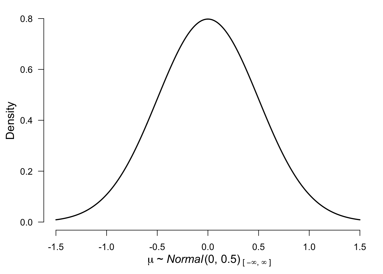
model 2
To add model 2 - we set the prior for the mu parameter to be treated as an alternative prior and the remaining priors treated as null priors.
fit <- update(fit,
              prior_mu         = prior("normal", parameters = list(mean = 0, sd = .5)),
              prior_tau_null   = prior("spike",  parameters = list(location = 0)),
              prior_omega_null = prior("spike",  parameters = list(location = 1)))
model 3 - 6
Let’s now add the remaining models.
### adding model 3
fit <- update(fit,
              prior_mu         = prior("normal",   parameters = list(mean = 0, sd = .5)),
              prior_tau        = prior("invgamma", parameters = list(shape = 1, scale = .15)),
              prior_omega_null = prior("spike",    parameters = list(location = 1)))

### adding model 4
fit <- update(fit,
              prior_mu         = prior("spike",     parameters = list(location = 0)),
              prior_tau        = prior("spike",     parameters = list(location = 0)),
              prior_omega      = prior("one.sided", parameters = list(steps = c(0.05, .10), alpha = c(1,1,1))))

### adding model 5
fit <- update(fit,
              prior_mu         = prior("normal",    parameters = list(mean = 0, sd = .5)),
              prior_tau        = prior("spike",     parameters = list(location = 0)),
              prior_omega      = prior("one.sided", parameters = list(steps = c(0.05, .10), alpha = c(1,1,1))))

### adding model 6
fit <- update(fit,
              prior_mu         = prior("normal",    parameters = list(mean = 0, sd = .5)),
              prior_tau        = prior("invgamma",  parameters = list(shape = 1, scale = .15)),
              prior_omega      = prior("one.sided", parameters = list(steps = c(0.05, .10), alpha = c(1,1,1))))
Note. Here we applied inverse-gamma (1, .15) prior distribution based on empirical heterogeneities (Erp et al., 2017) for the heterogeneity parameter tau in the random effects models (3, 6). For models assuming publication bias (4-6), we specified a one-sided three-step weight function differentiating between marginally significant and significant p-values.
summary results
summary(fit)## Call:
## RoBMA(t = df_simu$TE, n = df_simu$n, study_names = df_simu$studlab,
## priors_mu = NULL, priors_tau = NULL, priors_omega = NULL,
## priors_mu_null = prior("spike", parameters = list(location = 0)),
## priors_tau_null = prior("spike", parameters = list(location = 0)),
## priors_omega_null = prior("spike", parameters = list(location = 1)),
## control = list(silent = TRUE), seed = 12)
##
## Robust Bayesian Meta-Analysis
## Models Prior prob. Post. prob. Incl. BF
## Effect 5/6 0.833 0.816 0.888
## Heterogeneity 4/6 0.667 0.055 0.029
## Pub. bias 3/6 0.500 0.014 0.014
##
## Model-averaged estimates
## Mean Median 0.025 0.975
## mu 0.082 0.090 0.000 0.168
## tau 0.002 0.000 0.000 0.046
## omega[0,0.05] 1.000 1.000 1.000 1.000
## omega[0.05,0.1] 0.999 1.000 1.000 1.000
## omega[0.1,1] 0.998 1.000 1.000 1.000
## (Estimated omegas correspond to one-sided p-values)plot
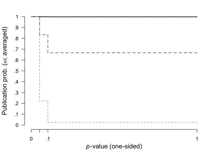
Here we plotted the prior (grey dashed lines) and posterior (black lines, with 95% CI) distribution for the weight function.
plot(fit, parameter = "omega", prior = TRUE)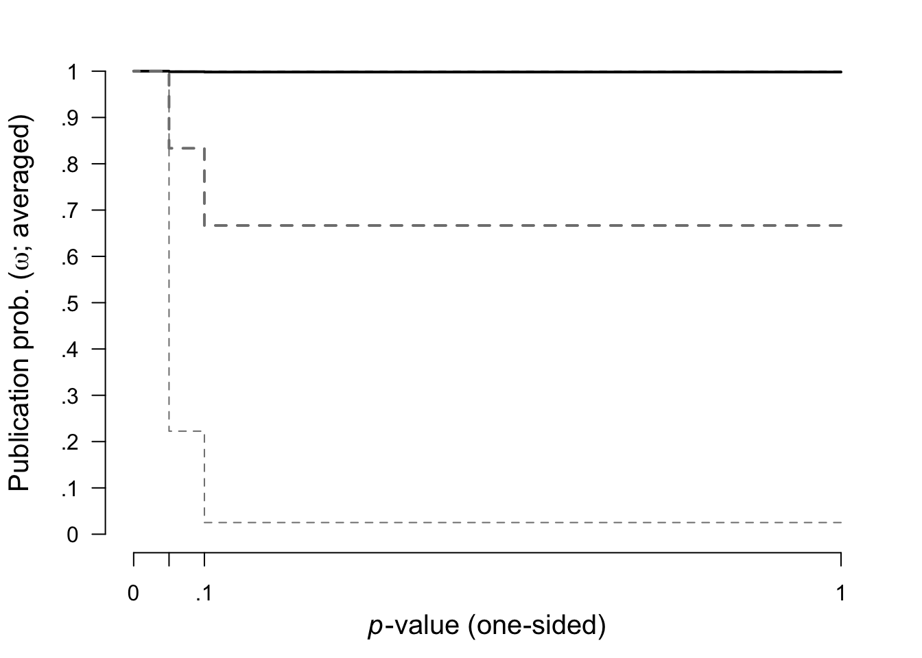
References
Citkowicz, M., & Vevea, J. L. (2017). A parsimonious weight function for modeling publication bias. Psychological Methods, 22(1), 28–41. https://doi.org/10.1037/met0000119
Du, H., Liu, F., & Wang, L. (2017). A Bayesian “fill-in” method for correcting for publication bias in meta-analysis. Psychological Methods, 22(4), 799–817. https://doi.org/10.1037/met0000164
Guan, M., & Vandekerckhove, J. (2016). A Bayesian approach to mitigation of publication bias. Psychonomic Bulletin & Review, 23(1), 74–86. https://doi.org/10.3758/s13423-015-0868-6
Maier, M., Bartoš, F., & Wagenmakers, E.-J. (2021). Robust Bayesian Meta-Analysis: Addressing Publication Bias with Model-Averaging. https://doi.org/10.31234/osf.io/u4cns
McShane, B. B., Böckenholt, U., & Hansen, K. T. (2016). Adjusting for Publication Bias in Meta-Analysis: An Evaluation of Selection Methods and Some Cautionary Notes. Perspectives on Psychological Science, 11(5), 730–749. https://doi.org/10.1177/1745691616662243
Rosenthal, R. (1979). The file drawer problem and tolerance for null results. Psychological Bulletin, 86(3), 638-641. doi:10.1037/0033-2909.86
Simonsohn, U., Nelson, L. D., & Simmons, J. P. (2014). P-curve: A key to the file-drawer. Journal of Experimental Psychology: General, 143(2), 534-547. doi:10.1037/a0033242
van Aert, R. C. M., & van Assen, M. A. L. M. (2020). Correcting for Publication Bias in a Meta-Analysis with the P-uniform* Method. https://doi.org/10.31222/osf.io/zqjr9
Van Erp, S., Verhagen, J., Grasman, R. P. P. P., & Wagenmakers, E.-J. (2017). Estimates of Between-Study Heterogeneity for 705 Meta-Analyses Reported in Psychological Bulletin From 1990–2013. Journal of Open Psychology Data, 5(1), 4. https://doi.org/10.5334/jopd.33